Linear Regression as the Simplest Classifier
Posted on Mon 24 February 2020 in Posts
In this post I wanted to describe a simple application of a linear least squares method to a problem of data classification. It is a naive approach and is unlikely to beat more sophisticated techniques like Logistic Regression, for instance.
Imports
Some imports we are going to need for this piece.
import numpy as np
import pandas as pd
from sklearn.linear_model import LinearRegression
from sklearn.neighbors import KNeighborsClassifier
from sklearn.metrics import accuracy_score
import matplotlib.pyplot as plt
%matplotlib inline

plt.style.use("ggplot")
Prepare the data
Data can be found here. The link also has information about the textbook with excellent theoretical background on much of Machine Learning (and Computational Statistics).
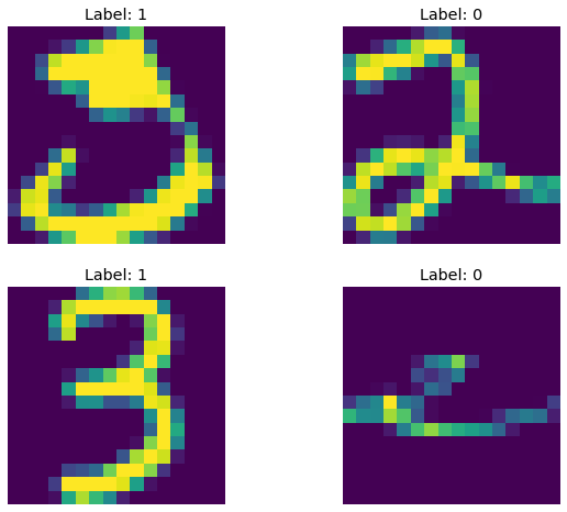
The data is a collection of hand-written digits. Each row of the data represents pixels of the image. For simplicity, we discard all labels except 2 and 3 making the problem a binary classification one (since only two labels are involved).
We load files with space character as a separator and no header
train = pd.read_csv('zip.train', sep=' ', header=None).drop(257, axis=1)
test = pd.read_csv('zip.test', sep=' ', header=None)
Select only required labels: (by default labels are read as float64 but we won't worry about that)
train = train.loc[train[0].isin([2.0, 3.0])].reset_index(drop=True)
test = test.loc[test[0].isin([2.0, 3.0])].reset_index(drop=True)
# convert types to int32 and replace labels with 0 and 1
train[0] = train[0].astype(np.int32).map({2: 0, 3: 1})
test[0] = test[0].astype(np.int32).map({2: 0, 3: 1})

X, y = train.iloc[:, 1:], train.iloc[:, 0]
X_test, y_test = test.iloc[:, 1:], test.iloc[:, 0]
X.info()
<class 'pandas.core.frame.DataFrame'>
RangeIndex: 1389 entries, 0 to 1388
Columns: 256 entries, 1 to 256
dtypes: float64(256)
memory usage: 2.7 MB
y.describe()
count    1389.000000
mean        0.473722
std         0.499489
min         0.000000
25%         0.000000
50%         0.000000
75%         1.000000
max         1.000000
Name: 0, dtype: float64
X_test.info()
<class 'pandas.core.frame.DataFrame'>
RangeIndex: 364 entries, 0 to 363
Columns: 256 entries, 1 to 256
dtypes: float64(256)
memory usage: 728.1 KB
y_test.describe()
count    364.000000
mean       0.456044
std        0.498750
min        0.000000
25%        0.000000
50%        0.000000
75%        1.000000
max        1.000000
Name: 0, dtype: float64
Some helper functions
def show_sample(data: pd.DataFrame):
    """Show 4 images from the dataset (random)."""
    sample = data.sample(4)
    fig, ax = plt.subplots(2, 2, figsize=(10, 8))
    for i in range(2):
        for j in range(2):
            ax[i, j].imshow(sample.iloc[2 * i + j, 1:].values.reshape(16, 16))
            ax[i, j].axis('off')
            ax[i, j].set_title(f'Label: {sample.iloc[2*i+j, 0]}')
    plt.show()


def raw2label(y_pred, threshold=0):
    """Convert raw label into a int label with a threshold."""
    return np.int32(y_pred > threshold)
show_sample(test)
Linear Regression fitting
We will approach the solution in the following way. Firstly, we will train a linear regression model on the available data (256 pixel intensity values). Note that the problem is high-dimensional and therefore it is impossible to visualize all of it at once.
However, the main idea of the linear regression based classifier remains simple: we find a hyperplane in the \(p+1=257\) dimensional space that fits the training data perfectly:
where \(X_i\) is the input column vector (features) with intercept (that is \(X_0=1\)):
\(\mathbf{X}\) is the matrix of features
and \(\beta=[\beta_0, \dots, \beta_p]\) is the vector of parameters
where \(\hat{\beta}\) is given by
We are projecting our training set \(\mathbf{X}\) orthogonally onto the hyperplane defined by \(\hat\beta\). We can then derive a classifier from there as follows: let us set up the threshold \(t\) such that if for a given unseen feature vector \(X_{test}\) the value \(y_{test}=X_{test}^T\hat\beta=\hat\beta_0+\sum\limits_{i=1}^p (X_{test})_i\hat\beta_i\) is greater than \(t\), we assign label 1, otherwise 0.
linreg = LinearRegression()
linreg.fit(X, y)
LinearRegression(copy_X=True, fit_intercept=True, n_jobs=None, normalize=False)
Train set predictions
y_true = y.copy().values
y_pred = linreg.predict(X)
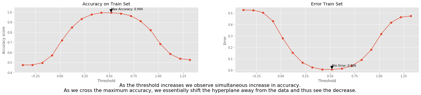
We select the threshold range between the minimum and maximum value of the predicted \(y\) with a step 0.1 and then check the accuracy for each threshold.
thresh_range = np.arange(y_pred.min(), y_pred.max(), 0.1)
train_acc_scores = []

for t in thresh_range:
    train_acc_scores.append(
        accuracy_score(y_pred=raw2label(y_pred, t), y_true=y_true))
fig, ax = plt.subplots(ncols=2, figsize=(24, 4))
ax[0].plot(thresh_range, train_acc_scores, '-o')
ax[0].set_title("Accuracy on Train Set")
ax[0].set_xlabel("Threshold")
ax[0].set_ylabel("Accuracy score")
ax[0].set_ylim([0.4, 1.05])
max_score = max(train_acc_scores)
max_loc = np.argmax(train_acc_scores)
ax[0].annotate(
    f'Max Accuracy: {max_score:.3f}',
    xy=(thresh_range[max_loc], max_score),
    xytext=(thresh_range[max_loc], max_score + 0.025),
    arrowprops=dict(facecolor='black', shrink=0.01),
)

ax[1].plot(thresh_range, 1 - np.array(train_acc_scores), '-o')
ax[1].set_title("Error Train Set")
ax[1].set_xlabel("Threshold")
ax[1].set_ylabel("Error")
min_score = min(1 - np.array(train_acc_scores))
min_loc = np.argmin(1 - np.array(train_acc_scores))
ax[1].annotate(
    f'Min Error: {min_score:.3f}',
    xy=(thresh_range[min_loc], min_score),
    xytext=(thresh_range[min_loc], min_score + 0.025),
    arrowprops=dict(facecolor='black', shrink=0.01),
)

fig.text(
    0.5,
    -0.1,
    'As the threshold increases we observe simultaneous increase in accuracy.\n'+\
    'As we cross the maximum accuracy, we essentially shift the hyperplane away from the data and thus see the decrease.',
    ha='center',
    fontsize=16);
Test set predictions
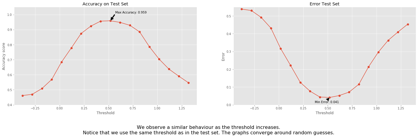
We can do similar analysis on the testing set.
y_true = y_test.copy().values
y_pred = linreg.predict(X_test)
test_acc_scores = []
for t in thresh_range:
    test_acc_scores.append(
        accuracy_score(y_pred=raw2label(y_pred, t), y_true=y_true))
fig, ax = plt.subplots(ncols=2, figsize=(24, 6))
ax[0].plot(thresh_range, test_acc_scores, '-o')
ax[0].set_title("Accuracy on Test Set")
ax[0].set_ylim([0.4, 1.05])
# ax[0].set_xticks(thresh_range)
ax[0].set_xlabel("Threshold")
ax[0].set_ylabel("Accuracy score")

max_score = max(test_acc_scores)
max_loc = np.argmax(test_acc_scores)
ax[0].annotate(
    f'Max Accuracy: {max_score:.3f}',
    xy=(thresh_range[max_loc], max_score),
    xytext=(thresh_range[max_loc] + 0.05, max_score + 0.05),
    arrowprops=dict(facecolor='black', shrink=0.01),
)

ax[1].plot(thresh_range, 1 - np.array(test_acc_scores), '-o')
ax[1].set_title("Error Test Set")
ax[1].set_xlabel("Threshold")
ax[1].set_ylabel("Error")
ax[1].set_ylim([0, 0.55])
min_score = min(1 - np.array(test_acc_scores))
min_loc = np.argmin(1 - np.array(test_acc_scores))
ax[1].annotate(
    f'Min Error: {min_score:.3f}',
    xy=(thresh_range[min_loc], min_score),
    xytext=(thresh_range[min_loc] - 0.15, min_score - 0.03),
    arrowprops=dict(facecolor='black', shrink=0.01),
)

fig.text(
    0.5,
    -0.1,
    'We observe a similar behaviour as the threshold increases.\n'+\
    'Notice that we use the same threshold as in the test set. '+\
    'The graphs converge around random guesses.',
    ha='center',
    fontsize=16);
percentage = np.unique(y_test, return_counts=True)[1]/len(y_test) # proportion of each label in the training set
print(f'Minimal accuracy on the left: {min(test_acc_scores)}, proportion of "0" labels in the data: {percentage[0]}')
print(f'Minimal accuracy on the right: {test_acc_scores[-1]}, proportion of "1" labels in the data: {percentage[1]}')
Minimal accuracy on the left: 0.46153846153846156, proportion of "0" labels in the data: 0.5439560439560439
Minimal accuracy on the right: 0.5467032967032966, proportion of "1" labels in the data: 0.45604395604395603
From the information above we learn that the model start to approximately randomly guess once the thresholds are too big or too small. On the left in is closer to guessing ones, on the right - zeros.
print(f"Labels from leftmost threshold:\n{raw2label(y_pred, threshold=thresh_range[0])}")
print(f"\n\nLabels from rightmost threshold:\n{raw2label(y_pred, threshold=thresh_range[-1])}")
Labels from leftmost threshold:
[1 1 1 1 1 1 1 1 1 1 1 1 1 1 1 1 1 1 1 1 1 1 1 1 1 1 1 1 1 1 1 1 1 1 1 1 1
 1 1 1 1 0 1 1 1 1 1 1 1 1 1 1 1 1 1 1 1 1 1 1 1 1 1 1 1 1 1 1 1 1 1 1 1 1
 1 1 1 1 1 1 1 1 1 1 1 1 1 1 1 1 1 1 1 1 1 1 1 1 1 1 1 1 1 1 1 1 0 1 1 1 1
 1 1 1 1 1 1 1 1 1 1 1 1 1 1 1 1 1 1 1 1 1 1 1 1 1 1 1 1 1 1 1 1 1 1 1 1 1
 1 1 1 1 1 1 1 1 1 1 1 1 1 1 1 1 1 1 1 1 1 1 1 1 1 1 1 1 1 1 1 1 1 1 1 1 1
 1 1 1 1 1 1 1 1 1 1 1 1 1 1 1 1 1 1 1 1 1 1 1 1 1 1 1 1 1 1 1 1 1 1 1 1 1
 1 1 1 1 1 1 1 1 1 1 1 1 1 1 1 1 1 1 1 1 1 1 1 1 1 1 1 1 1 1 1 1 1 1 1 1 1
 1 1 1 1 1 1 1 1 1 1 1 1 1 1 1 1 1 1 1 1 1 1 1 1 1 1 1 1 1 1 1 1 1 1 1 1 1
 1 1 1 1 1 1 1 1 1 1 1 1 1 1 1 1 1 1 1 1 1 1 1 1 1 1 1 1 1 1 1 1 1 1 1 1 1
 1 1 1 1 1 1 1 1 1 1 1 1 1 1 1 1 1 1 1 1 1 1 1 1 1 1 1 1 1 1 1]


Labels from rightmost threshold:
[0 0 0 0 0 0 0 0 0 0 0 0 0 0 0 0 0 0 0 0 0 0 0 0 0 0 0 0 0 0 0 0 0 0 0 0 0
 0 0 0 0 0 0 0 0 0 0 0 0 0 0 0 0 0 0 0 0 0 0 0 0 0 0 0 0 0 0 0 0 0 0 0 0 0
 0 0 0 0 0 0 0 0 0 0 0 0 0 0 0 0 0 0 0 0 0 0 0 0 0 0 0 0 0 0 0 0 0 0 0 0 0
 0 0 0 0 0 0 0 0 0 0 0 0 0 0 0 0 0 0 0 0 0 0 0 0 0 0 0 0 0 0 0 0 0 0 0 0 0
 0 0 0 0 0 0 0 0 0 0 0 0 0 0 0 0 0 0 0 0 0 0 0 0 0 0 0 0 0 0 0 0 0 0 0 0 0
 0 0 0 0 0 0 0 0 0 0 0 0 0 0 0 0 0 0 0 0 0 0 0 0 0 0 0 0 0 0 0 0 0 0 0 0 0
 0 0 0 0 0 0 0 0 0 0 0 0 0 0 0 0 0 0 0 0 0 0 0 0 0 0 0 0 0 0 0 0 0 0 0 1 0
 0 0 0 0 0 0 0 0 0 0 0 0 0 0 0 0 0 0 0 0 0 0 0 0 0 0 0 0 0 0 0 0 0 0 0 0 0
 0 0 0 0 0 0 0 0 0 0 0 0 0 0 0 0 0 0 0 0 0 0 0 0 0 0 0 0 1 0 0 0 0 0 0 0 0
 0 0 0 0 0 0 0 0 0 0 0 0 0 0 0 0 0 0 0 0 0 0 0 0 0 0 1 0 0 0 0]
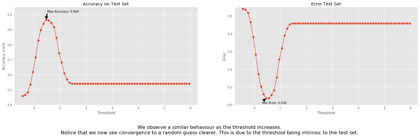
Let us use different thresholds for the testing set:
y_true = y_test.copy().values
y_pred = linreg.predict(X_test)
thresh_range = np.arange(y_pred.min(), y_pred.max(), 0.1)
test_acc_scores = []
for t in thresh_range:
    test_acc_scores.append(
        accuracy_score(y_pred=raw2label(y_pred, t), y_true=y_true))
fig, ax = plt.subplots(ncols=2, figsize=(24, 6))
ax[0].plot(thresh_range, test_acc_scores, '-o')
ax[0].set_title("Accuracy on Test Set")
ax[0].set_ylim([0.4, 1.05])
# ax[0].set_xticks(thresh_range)
ax[0].set_xlabel("Threshold")
ax[0].set_ylabel("Accuracy score")

max_score = max(test_acc_scores)
max_loc = np.argmax(test_acc_scores)
ax[0].annotate(
    f'Max Accuracy: {max_score:.3f}',
    xy=(thresh_range[max_loc], max_score),
    xytext=(thresh_range[max_loc] + 0.05, max_score + 0.05),
    arrowprops=dict(facecolor='black', shrink=0.01),
)

ax[1].plot(thresh_range, 1 - np.array(test_acc_scores), '-o')
ax[1].set_title("Error Test Set")
ax[1].set_xlabel("Threshold")
ax[1].set_ylabel("Error")
ax[1].set_ylim([0, 0.55])
min_score = min(1 - np.array(test_acc_scores))
min_loc = np.argmin(1 - np.array(test_acc_scores))
ax[1].annotate(
    f'Min Error: {min_score:.3f}',
    xy=(thresh_range[min_loc], min_score),
    xytext=(thresh_range[min_loc] - 0.15, min_score - 0.03),
    arrowprops=dict(facecolor='black', shrink=0.01),
)

fig.text(
    0.5,
    -0.1,
    'We observe a similar behaviour as the threshold increases.\n'+\
    'Notice that we now see convergence to a random guess clearer. '+\
    'This is due to the threshold being intrinsic to the test set.',
    ha='center',
    fontsize=16);
percentage = np.unique(y_test, return_counts=True)[1] / len(
    y_test)  # proportion of each label in the training set
print(
    f'Minimal accuracy on the left: {min(test_acc_scores)},'
    + f' proportion of "0" labels in the data: {percentage[0]}'
)
print(
    f"Labels from leftmost threshold:\n{raw2label(y_pred, threshold=thresh_range[0])}"
)

print(
    f'\n\nMinimal accuracy on the right: {test_acc_scores[-1]},' +
    f' proportion of "1" labels in the data: {percentage[1]}'
)
print(
    f"Labels from rightmost threshold: \n{raw2label(y_pred, threshold=thresh_range[-1])}"
)
Minimal accuracy on the left: 0.45879120879120877, proportion of "0" labels in the data: 0.5439560439560439
Labels from leftmost threshold:
[1 1 1 1 1 1 1 1 1 1 1 1 1 1 1 1 1 1 1 1 1 1 1 1 1 1 1 1 1 1 1 1 1 1 1 1 1
 1 1 1 1 0 1 1 1 1 1 1 1 1 1 1 1 1 1 1 1 1 1 1 1 1 1 1 1 1 1 1 1 1 1 1 1 1
 1 1 1 1 1 1 1 1 1 1 1 1 1 1 1 1 1 1 1 1 1 1 1 1 1 1 1 1 1 1 1 1 1 1 1 1 1
 1 1 1 1 1 1 1 1 1 1 1 1 1 1 1 1 1 1 1 1 1 1 1 1 1 1 1 1 1 1 1 1 1 1 1 1 1
 1 1 1 1 1 1 1 1 1 1 1 1 1 1 1 1 1 1 1 1 1 1 1 1 1 1 1 1 1 1 1 1 1 1 1 1 1
 1 1 1 1 1 1 1 1 1 1 1 1 1 1 1 1 1 1 1 1 1 1 1 1 1 1 1 1 1 1 1 1 1 1 1 1 1
 1 1 1 1 1 1 1 1 1 1 1 1 1 1 1 1 1 1 1 1 1 1 1 1 1 1 1 1 1 1 1 1 1 1 1 1 1
 1 1 1 1 1 1 1 1 1 1 1 1 1 1 1 1 1 1 1 1 1 1 1 1 1 1 1 1 1 1 1 1 1 1 1 1 1
 1 1 1 1 1 1 1 1 1 1 1 1 1 1 1 1 1 1 1 1 1 1 1 1 1 1 1 1 1 1 1 1 1 1 1 1 1
 1 1 1 1 1 1 1 1 1 1 1 1 1 1 1 1 1 1 1 1 1 1 1 1 1 1 1 1 1 1 1]


Minimal accuracy on the right: 0.5412087912087912, proportion of "1" labels in the data: 0.45604395604395603
Labels from rightmost threshold:
[0 0 0 0 0 0 0 0 0 0 0 0 0 0 0 0 0 0 0 0 0 0 0 0 0 0 0 0 0 0 0 0 0 0 0 0 0
 0 0 0 0 0 0 0 0 0 0 0 0 0 0 0 0 0 0 0 0 0 0 0 0 0 0 0 0 0 0 0 0 0 0 0 0 0
 0 0 0 0 0 0 0 0 0 0 0 0 0 0 0 0 0 0 0 0 0 0 0 0 0 0 0 0 0 0 0 0 0 0 0 0 0
 0 0 0 0 0 0 0 0 0 0 0 0 0 0 0 0 0 0 0 0 0 0 0 0 0 0 0 0 0 0 0 0 0 0 0 0 0
 0 0 0 0 0 0 0 0 0 0 0 0 0 0 0 0 0 0 0 0 0 0 0 0 0 0 0 0 0 0 0 0 0 0 0 0 0
 0 0 0 0 0 0 0 0 0 0 0 0 0 0 0 0 0 0 0 0 0 0 0 0 0 0 0 0 0 0 0 0 0 0 0 0 0
 0 0 0 0 0 0 0 0 0 0 0 0 0 0 0 0 0 0 0 0 0 0 0 0 0 0 0 0 0 0 0 0 0 0 0 0 0
 0 0 0 0 0 0 0 0 0 0 0 0 0 0 0 0 0 0 0 0 0 0 0 0 0 0 0 0 0 0 0 0 0 0 0 0 0
 0 0 0 0 0 0 0 0 0 0 0 0 0 0 0 0 0 0 0 0 0 0 0 0 0 0 0 0 0 0 0 0 0 0 0 0 0
 0 0 0 0 0 0 0 0 0 0 0 0 0 0 0 0 0 0 0 0 0 0 0 0 0 0 1 0 0 0 0]
K-Nearest Neighbors
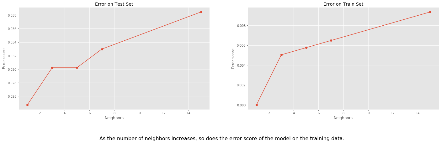
For this method, we consider different values of neighbors in each case. We begin with 1 neighbor per training point, which we expect to give a high accuracy since each point will roughly be each own neighborhood.
As the number of neighbors increases we will see a slight decrease in accuracy.
train_err_scores = []
test_err_scores = []

for k in [1, 3, 5, 7, 15]:
    knn = KNeighborsClassifier(n_neighbors=k)
    knn.fit(X, y)

    y_true = y.copy().values
    y_pred = knn.predict(X)

    train_err_scores.append(1 - accuracy_score(y_pred=y_pred, y_true=y_true))

    y_true = y_test.copy().values
    y_pred = knn.predict(X_test)
    test_err_scores.append(1 - accuracy_score(y_pred=y_pred, y_true=y_true))
fig, ax = plt.subplots(ncols=2, figsize=(24, 6))
ax[1].plot([1, 3, 5, 7, 15], train_err_scores, '-o')
ax[1].set_title("Error on Train Set")
ax[1].set_xlabel("Neighbors")
ax[1].set_ylabel("Error score")

ax[0].plot([1, 3, 5, 7, 15], test_err_scores, '-o')
ax[0].set_title("Error on Test Set")
ax[0].set_xlabel("Neighbors")
ax[0].set_ylabel("Error score")

fig.text(
    0.5,
    -0.1,
    'As the number of neighbors increases, so does the error score of the model on the training data.',
    ha='center',
    fontsize=16);
Conclusion
We applied two different classification methods for the data. Method 1 was based on the linear regression using least squares method. The second method was based on 5 different Nearest neighbor classifiers.
Each approach showed different results specific to assumptions underlying each model. Linear model assumes that the relationship between the label and pixel intensities is a high-dimensional linear function. Using various threshold we were able to show the change in hyperplane location relative to test and train data and how the accuracy scores (error scores) reflect this change.
For the k-NN model, we observed a similar behavior: going from few neighbors to more, we saw that the model is prone to the larger error. This is to be expected but not to say that 1 neighbor is necessarily better than 15 neighbors, since 1 neighbor case is overfitting the data. The data is very high-dimensional so it is harder to evaluate how many neighbors we should aim for here.