Three Ways to Deal With Imbalance
Posted on Mon 02 March 2020 in Posts
In this post, I put together an interesting example of what to do with imbalanced datasets and why precision and recall matter.
Introduction
The following is part of a Machine learning assignment I had to do while at CUNY. This particular example illustrates quite well the importance of understanding various measures of model quality such as accuracy, precision, recall, etc.
The idea is to predict whether a client will have a credit card default given some simple data. An insult to injury is a heavily imbalanced dataset: 97% of examples are "Yes"-labeled, making it difficult to train a good classifier.
We will dive into the solution, but first, some imports:
import pandas as pd
import seaborn as sns
import matplotlib.pyplot as plt
%matplotlib inline
import numpy as np
import gc
from sklearn.model_selection import train_test_split
from sklearn.metrics import confusion_matrix, precision_score, recall_score
from sklearn.linear_model import LogisticRegressionCV, LogisticRegression
plt.style.use('fivethirtyeight')
A plotting helper:
def plot_cm(y_pred, y_true):
    """Plot confusion matrix based on
       true vs. predicted values."""
    cm = confusion_matrix(y_true=y_true, y_pred=y_pred)
    prec = precision_score(y_true=y_true, y_pred=y_pred)
    rec = recall_score(y_true=y_true, y_pred=y_pred)
    sns.heatmap(cm, annot=True)
    plt.title(f"Precision: {prec:.2f}, Recall: {rec:.2f}")
Finally, reading the data:
df = pd.read_excel("Default.xlsx", header=0).iloc[:, 1:]

# convert strings to binary int32 0,1 values

df['default'] = df['default'].apply(lambda x: 0 if x == 'No' else 1).astype(
    np.int32)
df['student'] = df['student'].apply(lambda x: 0 if x == 'No' else 1).astype(
    np.int32)
X = df.drop(['default'], axis=1)
y = df['default']
To save memory: convert applicable columns from float64(double) to float32(float). This may help with much bigger datasets, this one is relatively small, though. Applicable here means max value of a column falls within the limits of the float32 range:
for column in df.columns:
    if df[column].values.max() < np.finfo(np.float32).max:
        if df[column].values.min() > np.finfo(np.float32).min:
            df[column] = df[column].values.astype(np.float32)
# garbage collector
gc.collect()
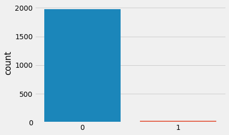
Let's look at the distribution of the target value:
ax = sns.countplot(data=df, x='default')
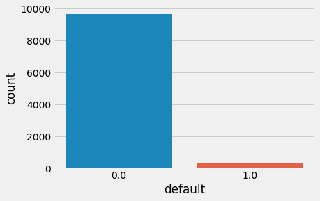
The histogram above verifies the problem: the data is highly imbalanced. To train a linear regression classifier, we will try to remedy the issue with three approaches:
- We sample a training, validation, and testing subsets in a stratified manner, that is, preserving the ratio between "0" and "1" labels.
- We will oversample the less represented class: "1", or "Yes"-labeled default examples.
- We will undersample the overrepresented class: "0".
Stratified Sampling
To sample in a way that the imbalance is preserved (stratified) we will pass an argument stratify to the train_test_split function from sklearn. Specifically, we will pass the column of labels df['default'] so that the function determines the exact distribution.
df_train, df_test, y_train, y_test = train_test_split(X,
                                                      y,
                                                      random_state=42,
                                                      stratify=df['default'],
                                                      train_size=0.6)

df_val, df_test, y_val, y_test = train_test_split(df_test,
                                                  y_test,
                                                  random_state=42,
                                                  stratify=y_test,
                                                  train_size=0.5)
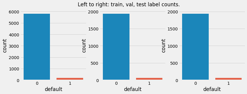
The plot below will illustrate the distribution of labels in the sampled data.
fig, ax = plt.subplots(ncols=3, figsize=(12, 4))
fig.suptitle("Left to right: train, val, test label counts.")
for i, data in zip(range(3), (y_train, y_val, y_test)):
    sns.countplot(x=data, ax=ax[i])
print(f'Train data to original dataset: {len(df_train)/len(X) * 100}%')
print(f'Validation data to original dataset: {len(df_val)/len(X) * 100}%')
print(f'Test data to original dataset: {len(df_test)/len(X) * 100}%')

print(f'\nNegative labels in original data: {len(X[y==0])/len(X) * 100 :.3}%')
print(f'Negative labels in train data: {(len(df_train[y_train==0])/len(df_train) * 100) :.3}%')
print(f'Negative labels in validation data: {(len(df_val[y_val==0])/len(df_val) * 100) :.3}%')
print(f'Negative labels in test data: {(len(df_test[y_test==0])/len(df_test) * 100) :.3}%')
Train data to original dataset: 60.0%
Validation data to original dataset: 20.0%
Test data to original dataset: 20.0%

Negative labels in original data: 96.7%
Negative labels in train data: 96.7%
Negative labels in validation data: 96.7%
Negative labels in test data: 96.7%
Oversampling
For oversampling we will use a package called imbalanced-learn available from PyPI. It has built-in classes for various over- and under-sampling methods. We will use basic RandomOverSampler and RandomUnderSampler classes.
The package is built with similarities to other sklearn conventions, so calling fit methods will give us the necessary results.
from imblearn.over_sampling import RandomOverSampler
ros = RandomOverSampler(random_state=42) # initialize
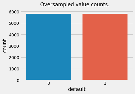
df_train_over, y_train_over = ros.fit_sample(
df_train, y=y_train) # resample training data
ax = sns.countplot(x=y_train_over) # plot value counts for the labels
t = plt.suptitle("Oversampled value counts.")
Underspamling
from imblearn.under_sampling import RandomUnderSampler
rus = RandomUnderSampler(random_state=42, ) # initialize
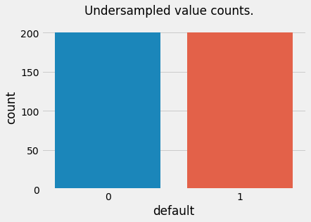
df_train_under, y_train_under = rus.fit_sample(df_train, y=y_train) # resample
ax = sns.countplot(x=y_train_under) # plot
t = plt.suptitle("Undersampled value counts.")
Train naively without stratification
Let us first train logistic regression model on a similarly split data without stratification.
df_train_naive, df_test_naive, y_train_naive, y_test_naive = train_test_split(
    X, y, random_state=42, train_size=0.6)

df_val_naive, df_test_naive, y_val_naive, y_test_naive = train_test_split(
    df_test_naive, y_test_naive, random_state=42, train_size=0.6)
logreg = LogisticRegression(penalty='none', max_iter=1e4, random_state=42)
logreg.fit(df_train_naive, y_train_naive)
y_pred = logreg.predict(df_val_naive)

plot_cm(y_val_naive, y_pred)
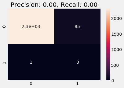
We observe zero precision and zero recall scores and the model overfits on the '0' class, which is expected and is bad.
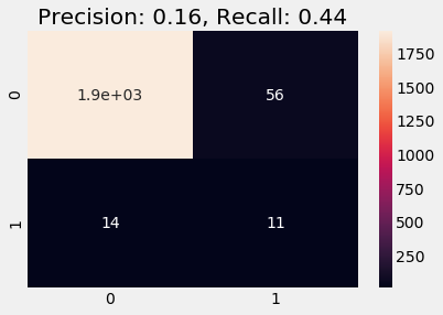
Train on Stratified
Below we train on the stratified data. We observe a better recall and precision scores and the predicted result on validation data follows the distribution of labels as in the training data (note that this heuristic is absolutely non-strict and does not necessarily indicate whether a model is good or bad).
logreg = LogisticRegression(penalty='none', max_iter=1e4, random_state=42)
logreg.fit(df_train, y_train)
y_pred = logreg.predict(df_val)

plot_cm(y_val, y_pred)

ax = plt.subplot()
ax = sns.countplot(y_pred, ax=ax)
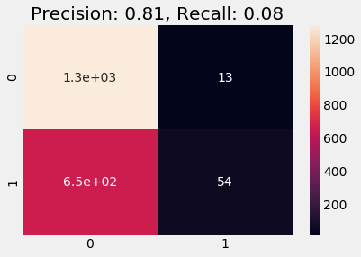
Train on Oversampled
When training on Oversampled data we get a very high precision score but lose the recall score.
logreg = LogisticRegression(penalty='none', max_iter=1e4, random_state=42)
logreg.fit(df_train_over, y_train_over)
y_pred = logreg.predict(df_val)

plot_cm(y_val, y_pred)
y_pred = logreg.predict(df_test)

plot_cm(y_test, y_pred)

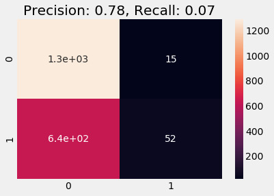
Train on Undersampled
A similar behavior occurs in the undersampled case, we see increase in Precision compared to naive and stratified cases, but both precision and recall are a bit lower that oversampled case.
logreg = LogisticRegression(penalty='none', max_iter=1e4, random_state=42)
logreg.fit(df_train_under, y_train_under)
y_pred = logreg.predict(df_val)

plot_cm(y_val, y_pred)
Conclusion
In this assignment, we considered a problem of default prediction for a credit card holder. We omitted most of preliminary data analysis and instead focused on basic model building for a highly imbalanced dataset. The proportion of negative labels is 97% out of all given data. Let us briefly outline meaning behind precision and recall scores.
Precision score shows the ratio of true positive predictions over all positive predictions regardless if they were true or false. If the number of true positive predictions is negligible compared to false positives then precision is low.
Recall score, on the other hand, shows the ratio of true positives versus the sum of true positive and false negative predictions. That is, if the prediction's number of true positive cases is trumped by the number of false negative cases, the recall score will be higher.
Card default is essentially the inability to pay off the card's balance. In this case, we are not willing to accept a false negative prediction: if we forecast that the default does not happen and in reality it does then we (the bank) are in the losing position. On the other hand, the false positive case does not affect us because in the worst case the cardholder pays off their debt and the default does not happen.
Since we want to be as effective as possible in our prediction, we must recommend a model with a higher recall score, which in this case is a stratified logistic recall score model.
logreg = LogisticRegression(penalty='none', max_iter=1e4, random_state=42)
logreg.fit(df_train, y_train)
y_pred = logreg.predict(df_val)

plot_cm(y_val, y_pred)
y_pred = logreg.predict(df_test)

plot_cm(y_test, y_pred)
