NumPy-Learn, A Homemade Machine Learning Library

Posted on Sun 14 June 2020 in Posts

In this post, I expand on a little class/self-teaching project that I did during the Spring 2020 semester.

NumPy-Learn: A Homemade Machine Learning Library

Organization

In this section we will discuss the main organization of the library:

How the layers are built
How loss functions work
How a stochastic gradient descent optimizer was built

After that, we introduce the class for building the neural net itself and explain how everything ties together. We conclude by performance analysis on a simple MNIST program.

Let us agree on convention similar to that of PyTorch library: we will call the main datatype Tensor instead of array, as follows:

from numpy import ndarray as Tensor

This is to adhere to accepted aesthetics of most modern neural network libraries and nothing more. All methods are purely using numpy or scipy.

Linear Layer

Inspired by PyTorch, the naming convention here is the preserved. The design of the layer is also similar to PyTorch: the class Linear will have a forward and a backward methods. The former will represent the forward pass, that is, the passing of the input data through the layer towards the next. The latter is responsible for backward propagation of the gradient.

Forward Pass

Linear layer essentially represents matrix multiplication of the input data $x$ by a weight matrix $W$ with addition of bias $b$:

$$\mathrm{L}(x) = xW + b.$$

We require that the size of the input data was of the format $batch\times input~features$, for instance if the input data has 784 pixel values, for a batch of 100 images the size of $x$ would be $100\times 784$ and the size of $W$ would be $784\times out~features$, while $b$ is of the shape $out~features\times 1$. Here we rely on numpy broadcasting the value of bias onto the resulting matrix $xW$ when adding $b$.

In code, we define it as follows:

def forward(self, x: Tensor) -> Tensor:
        self.input = x
        return x @ self.W + self.b

Gradient

In the forward pass, we computed the matrix product. Next, we need to evaluate the rate of change of the output of the current layer with respect to the input. Note, that due to the chain rule, the gradient flows from right (output) to left (input) as a product.

The backward method utilizes chainrule. It accepts the gradient from the layer $l+1$, uses it to find the derivatives of the current layer's output with respect to $W$ and $b$ and finally, passes it along multiplying by the derivative of its output w.r.t. $x$, the input.

Mathematically, this is the following:

The loss's derivatives w.r.t. weights are
$$\frac{\partial E}{\partial W^{l}_{ij}}=\sum\limits_{\text{input-output pair}}\delta^l_i out^{l-1}_j$$
.
Here, $\delta^l_i$ is the error of the $l$th layer for $i$th node:
$$\delta^l_i=g'_{out}(a_i^l)\sum\limits_k W^{l+1}_{ik}\delta^{l+1}_{k}$$
, where $g$ is the activation function.

These equations are written in a different shape convention, but we can take care of that in the code.

The derivative of $xW+b$ w.r.t. $W$ is $x^T$. The derivative of $xW+b$ w.r.t. to $b$ is an identity matrix. Therefore, let grad be the gradient (error) received from $(l+1)$th layer, then we can define the backward method as below:

def backward(self, grad: Tensor) -> Tensor:
        # input_feat by batch_size @ batch_size by out_features
        self.dydw = self.input.T @ grad
        # we sum across batches and get shape (out_features)
        self.dydb = grad.sum(axis=0)
        # output must be of shape (batch_size, out_features)
        return grad @ self.W.T

Now we are ready to present the fully defined Linear Layer code below:

import numpy as np
from numpy import ndarray as Tensor

class Linear:
    """A linear layer."""

    def __init__(self, in_features: int, out_features: int):
        """Initialize a linear layer with weights and biases."""
        self.W = np.random.randn(in_features, out_features)

        self.b = np.random.randn(out_features)

    def forward(self, x: Tensor) -> Tensor:
        """Compute forward pass, return W @ x + b.

        Arguments:
            W: the weight Tensor of shape (in_featuers, out_features)
            b: the bias vector of shape (out_features,)
            x: the input of shape (batch_size, in_features)

        Returns:
            A tensor of shape (batch_size, out_features)

        """
        self.input = x
        return x @ self.W + self.b

    def backward(self, grad: Tensor) -> Tensor:
        """Propagate the gradient from the l+1 layer to l-1 layer.

        Arguments:
            grad: the tensor gradients from the l+1 layer to be
                  propagated, shape: (batch_size, out_features).

        References:
            http://home.agh.edu.pl/~vlsi/AI/backp_t_en/backprop.html

        """
        # in_feat by batch_size @ batch_size by out_feat
        self.dydw = self.input.T @ grad
        # we sum across batches and get shape (out_features)
        self.dydb = grad.sum(axis=0)
        # output must be of shape (batch_size, out_features)
        return grad @ self.W.T

    def __call__(self, x: Tensor) -> Tensor:
        """Peform forward pass on `__call__`."""
        return self.forward(x)

    def __repr__(self) -> str:
        """Print a representation for Jupyter/IPython."""
        return f"""Linear Layer:\n\tWeight: {self.W.shape}"""\
            + f"""\n\tBias: {self.b.shape}"""

Layers with Activation Functions

We define separate layers for activation functions, similarly to the way PyTorch handles those. We only define two here: ReLU and Sigmoid.

ReLU is defined as

$$f(x) = \max\{0, x\}$$

and Sigmoid is defined as

$$\sigma(x) = \frac{1}{1+\exp(-x)}.$$

Their derivatives are defined as

$$(\nabla f)(t) = 0 \text{ if } t=0\text{, else }t$$

$$(\nabla \sigma)(t) = \sigma(t)(1-\sigma(t))$$

The respective classes are defined below

def sigmoid(x: Tensor) -> Tensor:
    """Calculate the sigmoid function of x."""
    return 1/(1+np.exp(-x))


def sigmoid_prime(x: Tensor) -> Tensor:
    """Calculate the d/dx of sigmoid function of x."""
    return sigmoid(x)*(1-sigmoid(x))

class ReLU:
    """ReLU class."""

    def __init__(self):
        """Initialize the ReLU instance."""

    def forward(self, x: Tensor) -> Tensor:
        """Compute the activation in the forward pass.

        Arguments:
            x: Tensor of inputs, shape (batch_size, in_features)

        Returns:
            Tensor of shape (batch_size, in_features)

        """
        return np.maximum(x, 0)

    def backward(self, grad: Tensor) -> Tensor:
        """Compute the gradient and pass it backwards.

        Arguments:
            grad: Tensor of gradients of shape (batch_size, out_features)

        Returns:
            Tensor of shape (batch_size, out_features)

        """
        return np.maximum(grad, 0)

    def __call__(self, x: Tensor) -> Tensor:
        """Peform forward pass on `__call__`."""
        return self.forward(x)

    def __repr__(self) -> str:
        """Print a representation of ReLU for Jupyter/IPython."""
        return """ReLU()"""


class Sigmoid:
    """Sigmoid class."""

    def __init__(self):
        """Initialize the instance.

        We add the main function for activation and its derivative function.
        """
        self.sigmoid = sigmoid
        self.sigmoid_prime = sigmoid_prime

    def forward(self, x: Tensor) -> Tensor:
        """Compute the activation in the forward pass.

        Arguments:
            x: Tensor of inputs with shape(batch_size, in_features)

        Returns:
            Tensor of shape(batch_size, in_features)

        """
        self.input = x
        return self.sigmoid(x)

    def backward(self, grad: Tensor):
        """Compute the gradient and pass it backwards.

        Arguments:
            grad: Tensor of gradients with shape(batch_size, out_features)

        Returns:
            Tensor of shape(in_features, out_features)

        """
        return self.sigmoid_prime(self.input) * grad

    def __call__(self, x: Tensor) -> Tensor:
        """Peform forward pass on `__call__`."""
        return self.forward(x)

    def __repr__(self) -> str:
        """Print a representation of Sigmoid for Jupyter/IPython."""
        return """Sigmoid()"""

In addition to Sigmoid and ReLU, we also import softmax activation function from scipy. In my experiments, I found that this is the most stable implementation, so I did not want to run into "not invented here" problem.

softmax is defined as follows:

$$\mathcal{S}(x)=\left[\frac{\exp(x_i)}{\sum\limits_{k}\exp(x_k)}\right], i=1..n,~x=[x_1, ... , x_n]$$

Softmax accepts a vector of network's output and converts it to a vector of probability values. For this function we need to use one-hot encoding.

from scipy.special import softmax as s
def softmax(x: Tensor) -> Tensor:
    """Calculate softmax using scipy."""
    return s(x, axis=1)

Loss Functions

We implement two loss functions here. We will implement Mean Squared Error Loss class and a Cross Entropy Loss class.

Mean Squared Error Loss

This is a very straight-forward loss function, it takes the output of the last layer of the neural network $\hat{y}$ and ccomputes:

$$\mathcal{L}(y, \hat{y}) = \frac{1}{2m}||y-\hat{y}||^2,$$

where $m$ is the size of $y$ and

$$\hat{y}$$

and

$$\vert\vert...\vert\vert$$

represents the vector norm (sum of squared component-wise differences). The gradient of this function for backpropagation is computed as

$$\nabla{\mathcal{L}}=\frac{1}{m}(y-\hat{y})$$

Cross Entropy Loss

Cross entropy loss function is defined as follows. Let $\hat{y}$ be the so-called ${logits}$, the outputs of the neural network. Then, we use softmax to calculate the probabilities $p=\mathcal{S}\left(\hat{y}\right)$. The cross entropy is

$$\mathcal{L}(y, \hat{y}) = -\sum\limits_{i} y_i \log p_i,$$

where $y_i$ is the true label vector.

To evaluate the gradient, consider the following argument

$$\nabla{\mathcal{L}}(y, \hat{y}) = -\sum\limits_i \frac{\partial \left(y_i \log [\mathcal{S}(x)]_i\right)}{\partial x_j}$$

where $x$ is the network's output. Continuing this, we obtain

$$\nabla{\mathcal{L}}(y, \hat{y}) = -\sum\limits_i y_i \frac{1}{p_i}\frac{\partial \mathcal{S}(x)_i}{\partial x_j}$$

To find the derivative of softmax, consider

$$\frac{\partial \mathcal{S}_i}{\partial x_j} = \frac{\partial}{\partial x_j}\left(\frac{\exp(x_i)}{\sum\limits_{k}\exp(x_k)}\right) = \frac{\frac{\partial\exp(x_i)}{\partial x_j} \sum\limits_{k}\exp(x_k) - \exp(x_i) \sum\limits_{k}\frac{\partial\exp(x_k)}{\partial x_j}}{\left(\sum\limits_{k}\exp(x_k)\right)^2},$$

$$\frac{\partial \mathcal{S}_i}{\partial x_j} = \frac{\exp(x_i)\delta_{ij} \sum\limits_{k}\exp(x_k) - \exp(x_i)\exp(x_j)}{\left(\sum\limits_{k}\exp(x_k)\right)^2},$$

$$\frac{\partial \mathcal{S}_i}{\partial x_j} = \frac{\exp(x_i)}{ \sum\limits_{k}\exp(x_k)}\delta_{ij} - \frac{\exp(x_i)}{\sum\limits_{k}\exp(x_k)}\frac{\exp(x_j)}{\sum\limits_{k}\exp(x_k)} = \mathcal{S}_i\delta_{ij} - \mathcal{S}_i \mathcal{S}_j.$$

We use $\delta_{ij}$ to represent Kronecker delta-symbol (essentially, identity matrix). Finally, we can interchange the notation $\mathcal{S}_i$ for $p_i$, since both represent the $i$th component of the softmax output (the probability)

$$\nabla{\mathcal{L}}(y, \hat{y}) = -\sum\limits_i y_i \frac{1}{p_i}p_i(\delta_{ij}-p_j) = - y_j + p_j\sum\limits_i y_i.$$

Recall, that the vector $y$ is one-hot encoded, therefore, the sum of its components $\sum\limits_i y_i=1$. Hence, we obtain

$$\nabla{\mathcal{L}}(y, \hat{y}) =p_j - y_j.$$

class Loss:
    """Placeholder class for losses."""

    def __init__(self):
        """Initialize the class with 0 gradient."""
        self.grad = 0.

    def grad_fn(self, pred: Tensor, true: Tensor) -> Tensor:
        """Create placeholder for the gradient funtion."""
        pass

    def loss_fn(self, pred: Tensor, true: Tensor) -> Tensor:
        """Create placeholder for the loss funtion."""
        pass

    def __call__(self, pred: Tensor, true: Tensor):
        """Calculate gradient and loss on call."""
        self.grad = self.grad_fn(pred, true)
        return self.loss_fn(pred, true)


class MSE(Loss):
    """Mean squared error loss."""

    def __init__(self):
        """Initialize via superclass."""
        super().__init__()

    def grad_fn(self, pred: Tensor, true: Tensor) -> Tensor:
        """Calculate the gradient of MSE.

        Args:
            pred: Tensor of predictions (raw output),
            shape (batch, )
            true: Tensor of true labels,
            shape (batch, )

        """
        return (pred - true)/true.shape[0]

    def loss_fn(self, pred: Tensor, true: Tensor) -> Tensor:
        """Calculate the MSE.

        Args:
            pred: Tensor of predictions (raw output),
            shape (batch,)
            true: Tensor of true labels (raw output),
            shape (batch,)

        """
        return 0.5*np.sum((pred - true)**2)/true.shape[0]

    def __repr__(self):
        """Put pretty representation in Jupyter/IPython."""
        return """Mean Squared Error loss (pred: Tensor, true: Tensor)"""


class CrossEntropyLoss(Loss):
    """CrossEntropyLoss class."""

    def __init__(self) -> None:
        """Initialize via superclass."""
        super().__init__()

    def loss_fn(self, logits: Tensor, true: Tensor) -> Tensor:
        """Calculate loss.

        Args:
            logits: Tensor of shape (batch size, number of classes),
            raw output of a neural network

            true: Tensor of shape (batch size,),
            a one-hot encoded vector

        """
        p = softmax(logits)
        return -np.mean(true * np.log(p))

    def grad_fn(self, logits: Tensor, true: Tensor) -> Tensor:
        """Calculate the gradient.

        Args:
            logits: Tensor of shape (batch size, number of classes),
            raw output of a neural network

            true: Tensor of shape (batch size, number of classes),
            a one-hot encoded vector

        """
        self.probabilities = softmax(logits)
        return self.probabilities - true

Building the Network

Here we describe the main class for our neural network. The main principle is simple, we pass a list of layers and initialize a class Network with two methods: forward and backward. The forward method performs the forward pass, that is, sends the input data through each layer. The backward method calls backward from each layer in the opposite direction (starting with the last layer). It uses the gradient of the lost function as its input.

from typing import List, Union

Layer = Union[Linear, ReLU, Sigmoid]


class Network:
    """Basic Neural Network Class."""

    def __init__(self, layers: List[Layer]):
        """Initialize the Netowrk with a list of layers."""
        self.layers = layers[:]

    def forward(self, x: Tensor):
        """Run the forward pass."""
        for l in self.layers:
            x = l(x)
        return x

    def backward(self, grad: Tensor):
        """Run the backward pass."""
        for l in self.layers[::-1]:
            grad = l.backward(grad)
        return grad

    def __call__(self, x: Tensor):
        """Run the forward pass on __call__."""
        return self.forward(x)

    def __repr__(self) -> str:
        """Print the representation for the network."""
        return "\n".join(l.__repr__() for l in self.layers)

Optimizers

Our main optimizer here is going to be Stochastic Gradient Descent. After we computed the backpropagation, for every layer in the network, we are going to update the weights. If the gradient is $\Delta w$ then the update rule is

$$w = w - \eta \Delta w - 2*\alpha w,$$

where $\eta$ is the learning rate and $\alpha$ is the $L^2$ regularization parameter. The code is presented below.

class SGD:
    """Stochastic Gradient Descent class."""

    def __init__(self, lr: float, l2: float = 0.):
        """Initialize with learning rate and l2-regularization parameter."""
        self.lr = lr
        self.l2 = l2

    def step(self, net: Network):
        """Perform optimization step."""
        for l in net.layers:
            if hasattr(l, 'dydw'):
                l.W = l.W - self.lr*l.dydw - 2 * self.l2 * l.W
            if hasattr(l, 'dydb'):
                l.b = l.b - self.lr*l.dydb - 2 * self.l2 * l.b

Training MNIST in Batches using MSE

In the code below, we create a training/validation loop. Each important point is commented.

from tqdm import auto
import numpy as np
import pandas as pd
from sklearn.metrics import accuracy_score
from sklearn.model_selection import train_test_split


def to_one_hot(vector: Tensor) -> Tensor:
    """Create one hot encoding of a vector."""
    oh = np.zeros((vector.shape[0], vector.max()+1))
    oh[np.arange(vector.shape[0]), vector] = 1
    return oh


# Load training data

train = pd.read_csv('mnist_train.csv', header=None).values[:, 1:]
train_label = pd.read_csv(
    'mnist_train.csv', header=None).values[:, 0]

# Create the basic network
net = Network(layers=[
    Linear(784, 128),
    ReLU(),
    Linear(128, 10),
])
# Initialize loss class
loss = MSE()

# Initialize the optimizer, learning rate is 0.0001
optim = SGD(1e-4)

# permform the train/val split
x_train, x_val, y_train, y_val = train_test_split(
    train.astype(np.float32) / 255,
    train_label.astype(np.int32),
    test_size=0.2, random_state=42)  # to_one_hot

# Convert labels to one-hot encodings
y_train = to_one_hot(y_train)
y_val = to_one_hot(y_val)

# batch size
batch_size = 100

# progress bar may not be visible in PDF mode, but it works in notebook or terminal mode
# we set it to 100 epochs here
progress_bar = auto.tqdm(range(100))
for epoch in progress_bar:
    # offset to iterate through batches
    offset = 0
    # initialize errors for validation and training
    val_err = 0
    err = 0
    while (offset+batch_size <= len(x_train)):
        # while we can move through batches, extract them
        data = x_train[offset:offset+batch_size, :]
        label = y_train[offset:offset+batch_size]
        # make prediction
        pred = net(data)
        # calculate loss (and average error)
        err += loss(pred, label)/(len(x_train)/batch_size)
        # begin backprop
        g = net.backward(loss.grad)
        # perform SGD step
        optim.step(net)
        # move to next batch
        offset += batch_size
    # reset offset for validation
    offset = 0
    while (offset+batch_size <= len(x_val)):
        # get validation data while we are not at the end
        val_data = x_val[offset:offset+batch_size, :]
        val_label = y_val[offset:offset+batch_size]
        # make prediction
        pred = net(val_data)
        # get loss and error
        val_err += loss(pred, val_label)/(len(x_val)/batch_size)
        # move offset to next batch
        offset += batch_size
        if (epoch) % 2 == 0:
            # update progress bar info
            progress_bar.set_postfix({"Mean_loss_train": err,
                                      "Mean_loss_val": val_err})

# Load test data and convert to one-hot
test = pd.read_csv('mnist_test.csv', header=None).values[:, 1:]
test_label = pd.read_csv('mnist_test.csv', header=None).values[:, 0]
test_label = to_one_hot(test_label)

# place offset and initialize error to 0
offset = 0
test_err = 0.
while (offset+batch_size <= len(test)):
    # get data batch
    data = test[offset:offset+batch_size, :]
    label = test_label[offset:offset+batch_size]
    # make prediction
    pred = net(data)
    # get error
    test_err += loss(pred, label)/(len(test)/batch_size)
    offset += batch_size


print(f"Test Error is {test_err:.2f} ...")

Test Error is 2643.26 ...

from sklearn.metrics import confusion_matrix
import seaborn as sns
import matplotlib.pyplot as plt
from IPython.display import set_matplotlib_formats
set_matplotlib_formats('retina')
plt.style.use('ggplot')
%matplotlib inline

y_true = test_label.argmax(1)
y_pred = net(test).argmax(1)
ax = plt.figure(figsize=(15, 7))
ax = sns.heatmap(confusion_matrix(y_true, y_pred), annot=True, fmt=".3f")
ax.set_xlabel("True")
ax.set_ylabel("Predicted")

Text(114.0, 0.5, 'Predicted')

png

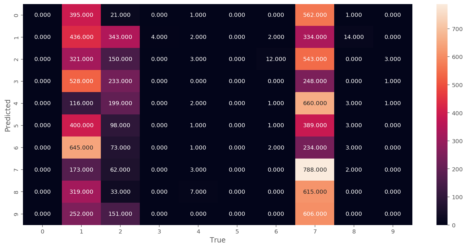
We can see from the confusion matrix above that the model performs poorly if the training is based on MSE. Let us try a different loss function: Cross Entropy loss.

Cross Entropy Training

"""Training example for a simple network with MNIST Dataset."""
from tqdm import auto
import numpy as np
import pandas as pd
from sklearn.metrics import accuracy_score
from sklearn.model_selection import train_test_split
from datatype import Tensor


def to_one_hot(vector: Tensor) -> Tensor:
    """Create one hot encoding of a vector."""
    oh = np.zeros((vector.shape[0], vector.max()+1))
    oh[np.arange(vector.shape[0]), vector] = 1
    return oh

# Load training data
train = pd.read_csv('mnist_train.csv', header=None).values[:, 1:]
train_label = pd.read_csv(
    'mnist_train.csv', header=None).values[:, 0]

# Create the network
net = Network(layers=[
    Linear(784, 128),
    Sigmoid(),
    Linear(128, 10),
])
# Initialize loss class
loss = CrossEntropyLoss()

# Initialize optimizer with regularization
optim = SGD(5e-2, 0.0001)

# split
x_train, x_val, y_train, y_val = train_test_split(
    train.astype(np.float32) / 255,
    train_label.astype(np.int32),
    test_size=0.2, random_state=42)  # to_one_hot

# to one-hot
y_train = to_one_hot(y_train)
y_val = to_one_hot(y_val)
batch_size = 100
progress_bar = auto.tqdm(range(200))

# this will be used later
accuracies: dict = {"train": [],
                    "val": [],
                    "test": []}
acc_train: list = []
acc_val: list = []

for epoch in progress_bar:
    offset = 0
    val_err = 0
    err = 0
    while (offset+batch_size <= len(x_train)):
        # grab the batch
        data = x_train[offset:offset+batch_size, :]
        label = y_train[offset:offset+batch_size, :]
        # I try to avoid a runtime warning (only happens in notebook, not sure why)
        try:
            pred = net(data)
        except RuntimeWarning:
            print(f"Runtime warning on {offset}")
        # get loss
        err += loss(pred, label)/(len(x_train)/batch_size)
        # backprop
        g = net.backward(loss.grad)
        # update weights
        optim.step(net)
        # next batch index
        offset += batch_size
        # keep scores
        acc_train.append(accuracy_score(
            label.argmax(axis=1),
            pred.argmax(axis=1)
        ))
    offset = 0
    while (offset+batch_size <= len(x_val)):
        # get validation data
        val_data = x_val[offset:offset+batch_size, :]
        val_label = y_val[offset:offset+batch_size]
        # predict
        pred = net(val_data)
        # get loss
        val_err += loss(pred, val_label)/(len(x_val)/batch_size)
        # next batch index
        offset += batch_size
        # keep scores
        acc_val.append(accuracy_score(
            val_label.argmax(axis=1),
            pred.argmax(axis=1)
        ))
    if (epoch) % 2 == 0:
        # update progress bar
        progress_bar.set_postfix({"loss_train": err,
                                  "loss_val": val_err,
                                  "acc_val": np.mean(acc_val)})
    # keep scores for visualization
    accuracies['train'].append(np.mean(acc_train))
    accuracies['val'].append(np.mean(acc_val))
    acc_train = []
    acc_val = []

# Load test data and convert to one-hot
test = pd.read_csv('mnist_test.csv', header=None).values[:, 1:]
test_label = to_one_hot(pd.read_csv(
    'mnist_test.csv',
    header=None).values[:, 0])


offset = 0
test_err = 0.
while (offset+batch_size <= len(test)):
    # get batch
    data = test[offset:offset+batch_size, :]
    label = test_label[offset:offset+batch_size]
    # predict
    pred = net(data)
    # get loss
    test_err += loss(pred, label)/(len(test)/batch_size)
    # offset
    offset += batch_size
    # get scores
    accuracies['test'].append(accuracy_score(
        label.argmax(axis=1),
        pred.argmax(axis=1)
    ))

print(f"Average Test Accuracy: {np.mean(accuracies['test']):.2f}")

Average Test Accuracy: 0.95

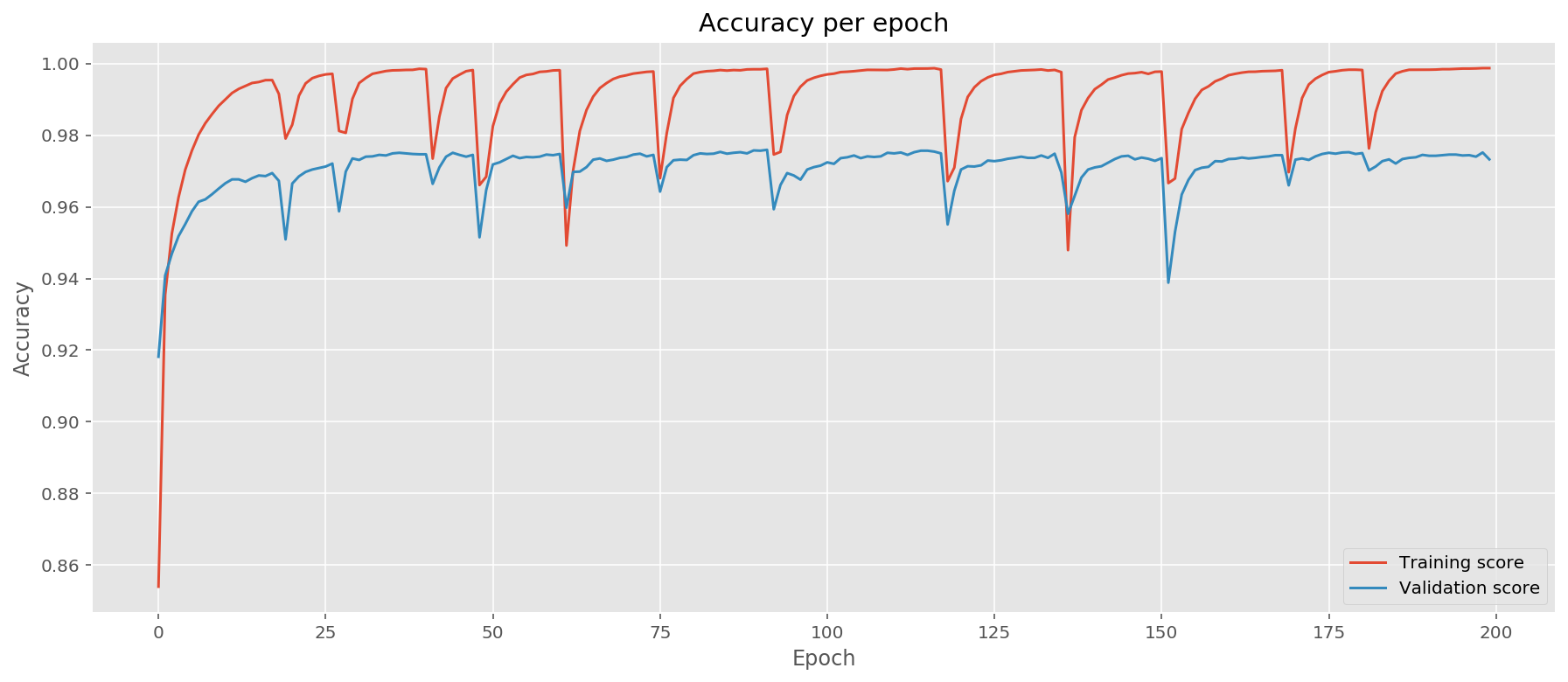
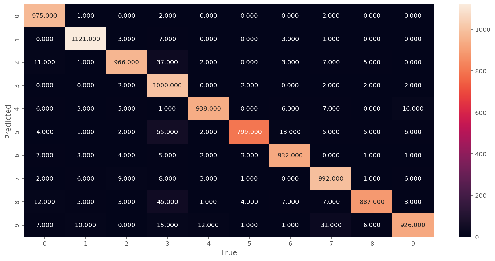
Let us plot the evolution of accuracies during testing and confusion matrix. For a higher performing model we expect to see the confusion matrix consolidate results on the diagonal:

fig = plt.figure(figsize=(15, 6))
_ = plt.plot(accuracies['train'], label="Training score")
_ = plt.plot(accuracies['val'], label="Validation score")
_ = plt.xlabel("Epoch")
_ = plt.ylabel("Accuracy")
_ = plt.title("Accuracy per epoch")
_ = plt.legend()

png

y_true = test_label.argmax(1)
y_pred = net(test).argmax(1)
_ = plt.figure(figsize=(15, 7))
ax = sns.heatmap(confusion_matrix(y_true, y_pred), annot=True, fmt=".3f")

_=ax.set_xlabel("True")
_=ax.set_ylabel("Predicted")

png

Conclusion

We implemented a neural network class that supports several activation functions. We followed here a design pattern based on PyTorch deep learning package. We implemented linear (fully-connected) layer, ReLU and Sigmoid layer. Each layer includes a backpropagation function backward that sends the gradient from the output back to input. As a result we were able to use a Cross Entropy Loss function to train a handwritten digit classifier with 95% accuracy on the test set. Notice that on the graph we observe a pattern of periodically dropping accuracy. I assume this is due to internal structure of the loss landscape: we repeatedly "walk" out of the minimum region and then "walk" back in during the SGD.

Using the Mean Squared Error loss function did not yield a productive result here, however, while developing this library, I observed that if I train on a small sample of data (i.e. 50 items or less), the model was able to learn the underlying data representations very well and was able to over fit. This is one the tests usually performed on new architectures in order to check if the model can learn at all. This, unfortunately, did not scale in case of MSE but it did for Cross Entropy Loss.

The overall structure of the project is posted on my github page