Simulating Textbook Probability Problems in Julia
Posted on Mon 07 February 2022 in Posts
Introduction
I am fascinated by the concept of Monte-Carlo simulation: you can, in principle, simulate random events and see how these simulations differ from reality (on a small scale, at least!)
Here I would like to show a couple of simple probability theory textbook problems and my attempt at simulating them in Julia.
I will make sure to include cool pictures!
Problem 1:
Here is the first problem's setting (from M. Baron's "Porbability and Statistics for Computer Science", 3rd edition, Question 2.5):
There are 3 independent computer hardware tests; probabilities of each test being positive are 0.2, 0.3, 0.5. What is the probability that at least one is correct?
Theoretical Solution
How would we solve this on paper? Probability of "at least" is always 1 minus probability of "neither". That is,
The latter value is, of course, a product of three probabilities of independent events. If our tests are \(A,~B,~C\) with complements (opposites) \(A^c,~B^c,~C^c\), then:
Note that \(\mathbb{P}(A^c) = 1 - \mathbb{P}(A)\) and same for \(B,~C\). Thus, the true answer will be
This value equals 0.72, let's keep that in mind.
Monte-Carlo Simulation
Let's now go ahead and simulate this process. To do this, we will use Julia 1.7.1 and Distributions package. Each test is a binary Bernoulli random variable, true or false with given probability:
using Distributions

test_1 = Bernoulli(0.2)
test_2 = Bernoulli(0.3)
test_3 = Bernoulli(0.5)
Let's define a function that takes in 3 tests and number of experiments (independent simulations).
This function will iterate for the number of experiments n_experiments and sample each test independently via rand function of Julia. We will check if any of those samples returns true and if that's the case we will increase the counter of "successful" experiments by 1.
At the end, the function will return the relative frequency of successes out of all experiments.
function simulation(test_1, test_2, test_3, n_experiments::Int)
    successful = 0
    for exp in 1:n_experiments
        if any([rand(test_1), rand(test_2), rand(test_3)])
            successful += 1
        end
    end
    return successful / n_experiments
end
Let's run this for several rounds of \(10^2\), \(10^3\), \(10^4\), \(10^6\), and \(10^9\) experiments. The results are as follows:
Show code
julia> rounds = [100, 1000, 10^4, 10^6, 10^9]
julia> results = [simulation(test_1, test_2, test_3, r) for r ∈ rounds]
5-element Vector{Float64}:
 0.69
 0.734
 0.7218
 0.720412
 0.719976697
Good news is that this approach is converging to the correct value of 0.72!
Now let's try to visualize it.
Show code
to_plot = [simulation(test_1, test_2, test_3, r) for r ∈ 1:10000]
@gif for i ∈ 1:10000
plot(to_plot[1:i])
end
As you can see from the GIF below, the model starts to jump around 0.72 after about 200 iterations. Recall that 0.72 is our predicted answer!

Problem 2: Rolling 3 Dice
Assume we have 3 dice that are rolled independently. What is the probability that one of 3 numbers is "6" and the other two are non-equal numbers between 1 and 5?
To get a theoretical answer, let's assume first that "6" is the first number. The other two are a pair of distinct numbers between 1 and 5. there are 5 options for the first and 4 options for the second, hence 20 combinations total. Now, "6" can be in the second and thirds positions, therefore we have a total of 20 + 20 + 20 different options that favor us.
The sample space contains all pairs of three numbers between 1 and 6 of which there are \(6^3\). Hence the answer is \(\frac{60}{216}\approx 0.27\)
To simulate it, we use the following function (not the most efficient implementation!):
function simulation(n_experiments::Int = 100)
    dice = [DiscreteUniform(1, 6) for i in 1:3]
    successes = 0
    for trial in 1:n_experiments
        experiment = rand.(dice)
        one_six = sum(r == 6 for r in experiment) == 1
        others = filter(num -> num != 6, experiment)
        no_duplicates = length(Set(others)) == 2
        if no_duplicates
            if one_six
                successes += 1
            end
        end
    end
    return successes / n_experiments
end
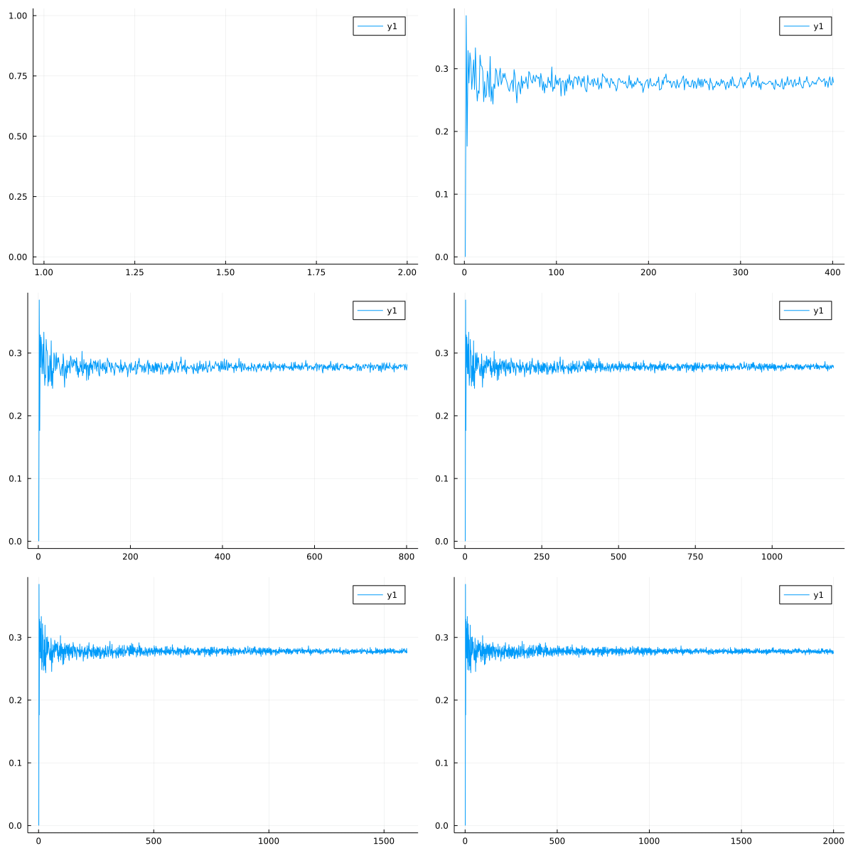
Let us create a similar GIF plot for the success frequency:
Show code
results = simulation.(1:25:50000)
@gif for i ∈ 1:length(results)
plot(results[1:i])
end
The gif of the frequency is below:

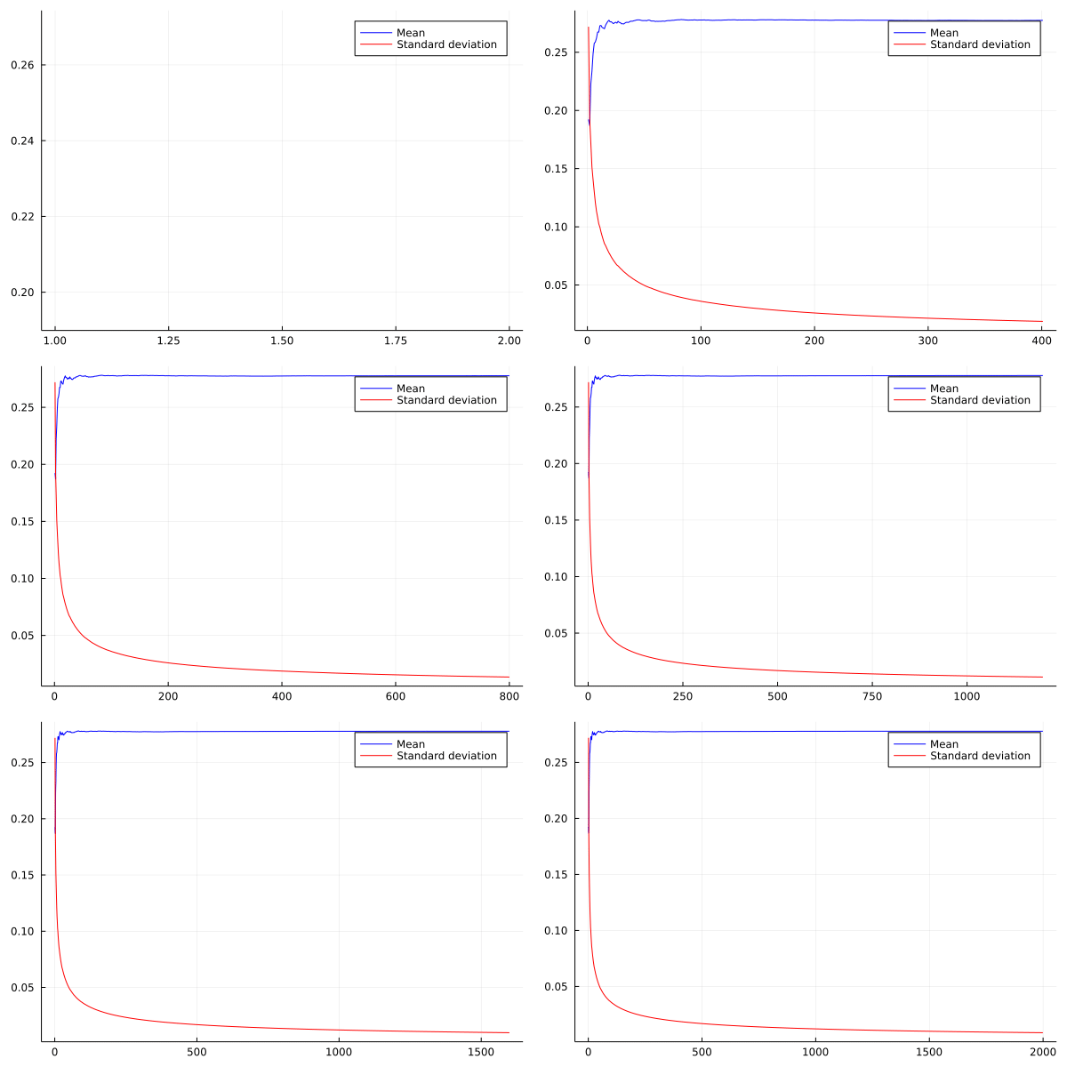
Let's also look at the average as we increase the number of iterations:
Show code
means = [mean(results[1:i]) for i ∈ 2:length(results)]
stddevs = [std(results[1:i]) for i ∈ 2:length(results)]

@gif for i ∈ 1:length(results)-1
       plot(means[1:i], label = "Mean", color=:blue)
       plot!(stddevs[1:i], label="Standard deviation", color=:red)
end

We see that those are immediately converging. The mean is around 0.277, which is our true value.